A tool for interpolating 2D seismic velocity data from sparse velocity analysis found in seismic sections.
Go to Installation to see how to install VelRecover.

Quick Start Guide
Key Features
- Velocity data interpolation - Create complete velocity models from sparse picks
- Multiple interpolation methods - Linear, logarithmic, RBF, and two-step approaches
- User-friendly GUI - Simple workflow with visual guidance
- Multiple export formats - Save as text or binary formats
Basic Workflow
- Load velocity data: Import from text files (Trace, TWT, Velocity)
- Load SEGY file: Provide spatial context
- Edit data: Remove outliers, edit velocity picks or add new ones
- Interpolate: Generate a complete velocity field
- Apply smoothing: Use Gaussian blur to eliminate artifacts (optional)
- Export results: Save in various formats for further use
First Run Setup
When you run VelRecover for the first time, you'll need to set up your data directory:
- The First Run Dialog will appear asking you to select a location for your data
- Choose a location with sufficient disk space for your project files
- Click "OK" to confirm your selection
- VelRecover will create the necessary folder structure and copy example files
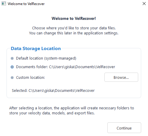
First Run Setup Dialog
Preparation
Before beginning the interpolation process, organize your files and understand the data requirements:
1. Folder Structure
VelRecover organizes your data in the following directories:
SEGY/- Store seismic SEGY filesVELS/RAW/- Store input velocity data filesVELS/2D/- Store interpolated velocity models (.txt or .bin)
2. Input Data Format
- Velocity data files: Text files with 3 columns
- SEGY files: Standard SEG-Y format (.segy) for the corresponding seismic line
| CDP | TWT | Velocity |
|---|---|---|
| 100 | 500 | 1500 |
| 200 | 1000 | 1800 |
| 300 | 1500 | 2100 |
Step 1: Loading Velocity Data
- From the Welcome screen, click the "New Velocity Field" button
- In the Load Data tab, click "Load SEGY File" to provide spatial context for the interpolation
- Click "Load Text File" to select your velocity data file (formats: .dat, .txt, .tsv, .csv)
- The velocity picks will be loaded and displayed over the SEG-Y file
- Click "Next" to proceed to the Edit tab
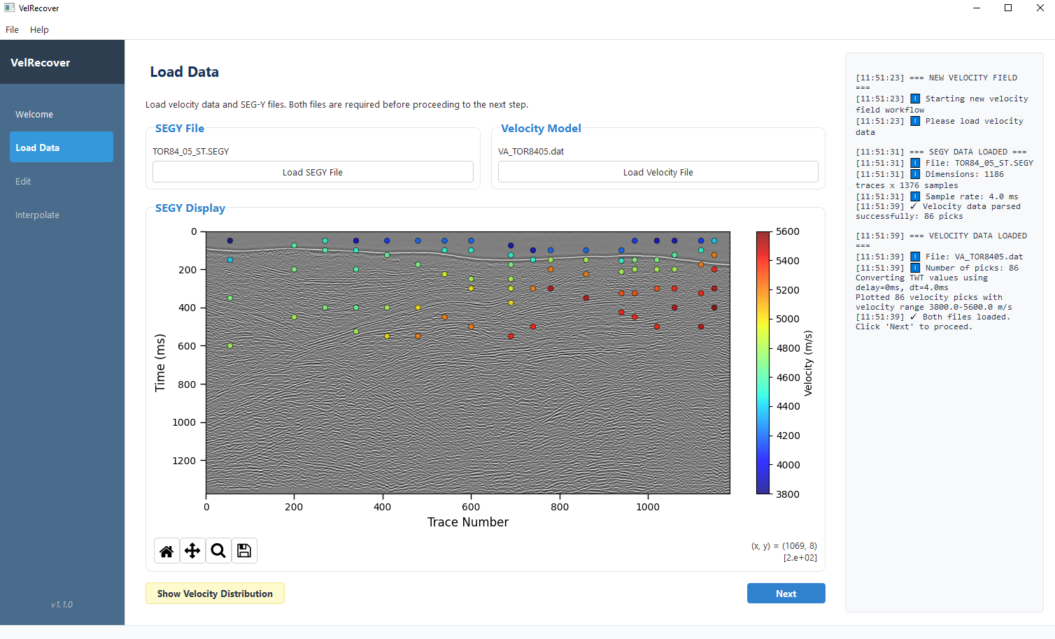
Window for loading velocity data and SEGY files
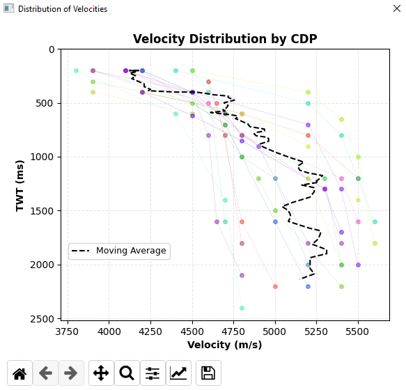
Velocity distribution plot showing the velocity values vs two-way-time for each trace or CDP in the text file MISSING REGRESSIION
Step 2: Editing Velocity Data
In this step, you'll review and edit your velocity data to remove outliers or incorrect velocity picks. You can also add new picks to improve the accuracy of the model:
- Click "Apply Time Shift" to shift all your velocity picks along the time axis
- Click "Edit pick" to select a pick and edit its velocity value
- Click "Add pick" to add a new velocity pick at the selected Trace and TWT
- Click "Delete pick" to remove a selected velocity pick
- Click "Save edits" and select where you want to save the new velocity picks, then click "Next" to proceed to the Interpolate tab
- Click "Continue without edits" and then "Next" if you don't want to make any edits
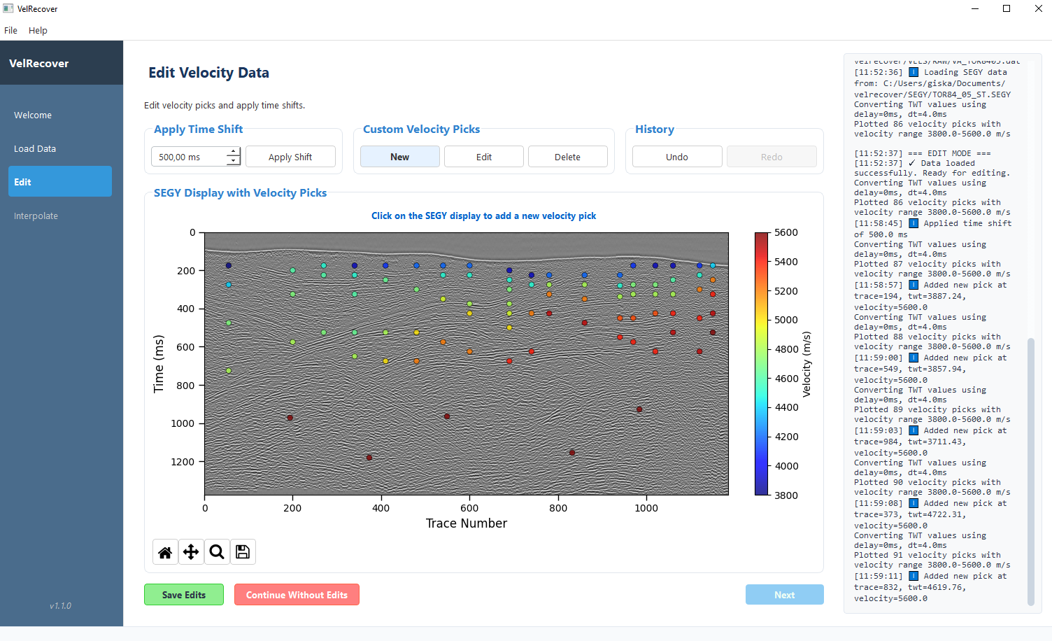
Data editing interface for cleaning velocity data. New picks has been added at the seismic section bottom.
Step 3: Interpolation
Once your data is cleaned, you can perform the interpolation to generate a complete velocity field:
- In the Interpolate tab, select the interpolation method from the dropdown menu:
- Linear Best Fit: Simple linear based on the linear best fit for all velocity picks (V=V0+kt)
- Linear Custom: Create a custom linear model by defininf the V0 and k coefficients (V=V0+kt)
- Logarithmic Best Fit: Model based in the natural logarithmic best fit for all velocity picks
- Logarithmic Custom: Create a custom logarithmic model by defining the V0 and k coefficients (V=V0+kln(t)
- RBF (Radial Basis Function): Creates smooth transitions between points
- Two-Step: First interpolates each trace with velocity picks using RBF interpolation and then fills missing traces with nearest neighbor interpolation
- Click "Run Interpolation" to process the data
- The resulting velocity field will be displayed as a color-coded grid
- For smoother results, enter a Gaussian blur value (1-100) and click "Run Interpolation" again
- Click "Reset" to delete the current interpolation
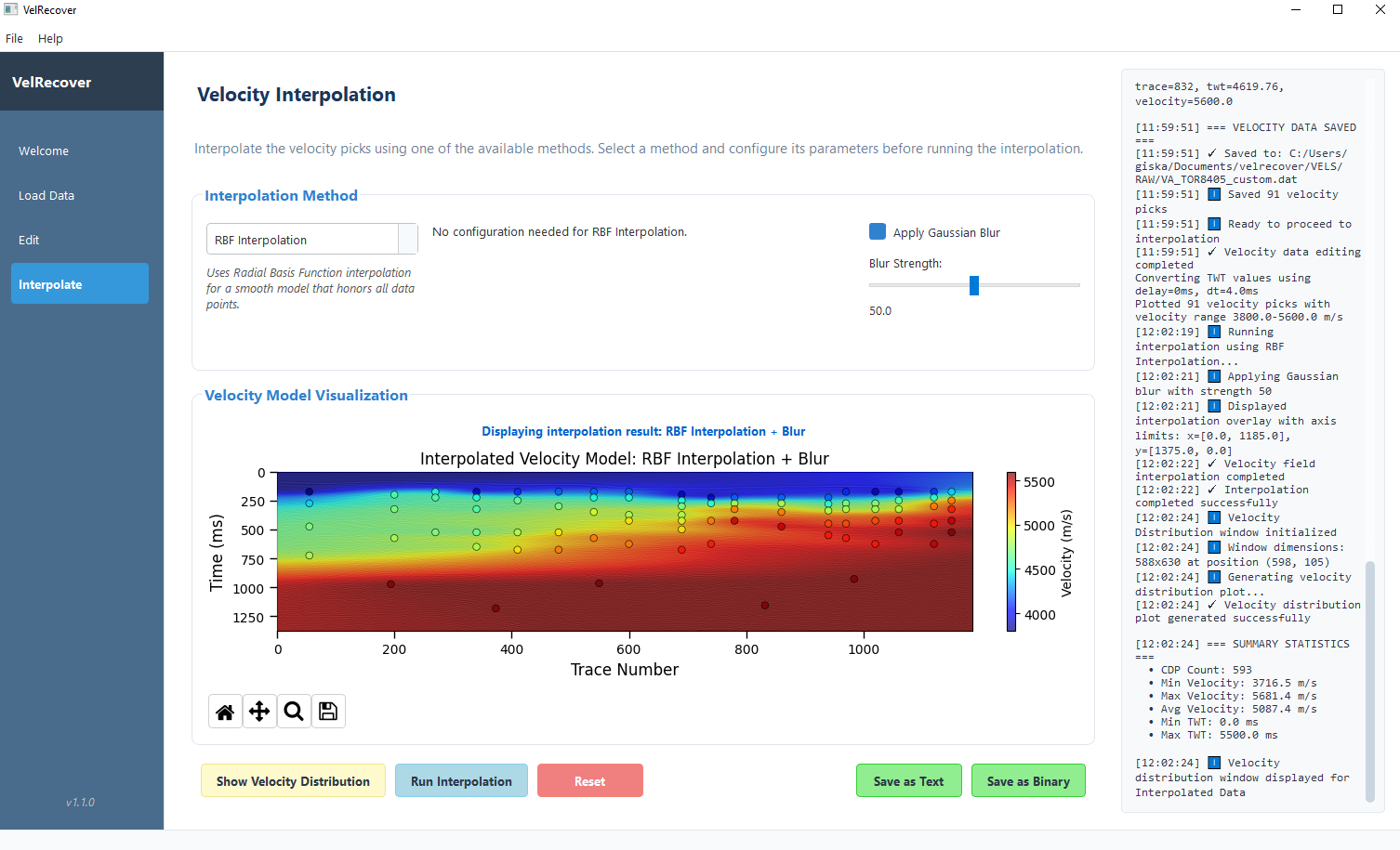
Interpolation interface showing the velocity field visualization
After interpolation, you can export your velocity field in various formats:
- Save Data as TXT: Exports as a text file with X, Y coordinates and CDP, TWT, Velocity values
- Save Data as BIN: Exports in binary format (float32) as a velocity grid (TWT, CDP)
Interpolation Methods
Linear Models
- Description: Simple linear based on the linear best fit for all velocity picks (V=V0+kt)
- Best for: Simple velocity fields with gradual changes
- Advantages: Fast computation, predictable results
- Limitations: May not accurately represent natural velocity trends with depth
Logarithmic Models
- Description: Model based in the natural logarithmic best fit for all velocity picks
- Best for: Simple velocity fields with gradual changes but accounting for compactation
- Advantages: Better represents natural velocity behavior
- Limitations: May create unusual values at the surface, apply gaussian blur for a better result
RBF (Radial Basis Function)
- Description: Uses radial basis functions to create smooth interpolation surfaces
- Best for: Complex velocity fields with irregular sampling
- Advantages: Creates natural-looking transitions between sparse points
- Limitations: Computationally intensive for large datasets. May create anomalous gradients if no picks are present. Suggest creating new picks to guide the interpolation at depth.
Two-Step Interpolation
- Description: Combines horizontal and vertical interpolation approaches
- Best for: Areas with complex geology and lateral velocity variations
- Advantages: Handles both lateral and vertical trends effectively
- Limitations: Most computationally intensive method
Gaussian Blur
- Description: Post-processing smoothing filter to reduce artifacts
- Best for: Smoothing results from any interpolation method
- Usage: Apply after interpolation with strength from 1 (minimal) to 100 (maximum)
- Caution: High values can over-smooth and remove legitimate velocity features
Troubleshooting
Use this guide to resolve common issues when using VelRecover:
Data loading issues
- Ensure your text file has 3 columns: CDP, TWT, Velocity
- Leave just one line of comments or headers
- Verify that all values are numeric with no text characters
Interpolation artifacts
- Edit out any obvious outliers in your velocity data
- Try a different interpolation method more suitable for your data
- Apply Gaussian blur to smooth out small-scale artifacts
Log Files
VelRecover creates log files for each session in the data directory. These contain process details and error messages that can help diagnose issues.
Frequently Asked Questions
What's the best interpolation method for typical seismic velocity data?
The best method depends on your specific data characteristics:
- For simple geology: Logarithmic Best Fit often provides good results as it mimics natural velocity increase with depth
- For complex geology: The Two-Step method usually provides the most realistic results as it honors both vertical and lateral variations
- For sparse data: RBF can work well but may need smoothing with Gaussian blur
We recommend trying multiple methods and comparing the results to determine which best represents your geological understanding of the area.
How many velocity picks do I need for a good model?
For a typical 2D seismic section:
- Minimum: At least 3-5 velocity picks per trace at different depths
- Recommended: One velocity pick every 10-20 CDPs horizontally, with 5-10 picks vertically distributed through the time range
- For areas with complex velocity variations, increase pick density accordingly
It's more important to have good coverage at depth intervals where velocity changes significantly than to have a large number of picks.
What Gaussian blur value should I use?
Gaussian blur smoothing guidelines:
- Minimal smoothing (1-10): Use for well-sampled data with minimal artifacts
- Moderate smoothing (10-30): Recommended for most datasets to remove small inconsistencies
- High smoothing (30-70): Use when interpolation results show significant artifacts
- Maximum smoothing (70-100): For very sparse data with severe interpolation artifacts
Start with a value around 20 and adjust based on visual inspection of the velocity field. Higher values may remove legitimate velocity features, so use with caution.
Can I export my velocity model for use in other software?
Yes, VelRecover offers multiple export options compatible with various software:
- Text format (.txt): CSV-style format with CDP, TWT, and Velocity values that can be imported into most interpretation software including Petrel, Kingdom, and OpendTect
- Binary format (.bin): Direct binary grid of velocity values (float32) organized by TWT and CDP, primarily for use with Seismic Unix processing tools
For other formats, you can use the text export and convert it using Python or other tools to match your specific software requirements.